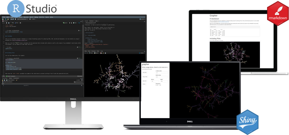
Shiny
grapher has a number of functions to work hand in hand with Shiny.

In Rmarkdown there is nothing specific to note, create visualisation in code chunks as you normally would. If you want to save the visualisation you can use save_graph_html.
A basic Shiny app with grapher might look like this.
library(shiny)
library(grapher)

g <- make_data(500)

ui <- fluidPage(
  graphOutput("graph", height = "100vh")
)

server <- function(input, output){
  output$graph <- render_graph({
    graph(g) %>%
      graph_layout_stable(ms = 3000)
  })
}

shinyApp(ui, server)
Events
Events send data from the JavaScript visualisation back to R to let you know how user interact with the graph. You can capture the following events:
- Node click
- Node double click
- Node hover
By default none of this data is sent back to the shiny server, you need to use one of the capture_* functions to do so. You can then get that event data as a usual input, combining the id of the graph you want and the name of the event you want to capture.
graphId_node_clickgraphId_node_double_clickgraphId_node_hover
Note that the reason this is not enabled by default is that it can be costly depending on the number of events triggered and the amount of data these carry, they can greatly slow down the visualisation. One should refrain from using capturing node hover on larger graphs.
An example of an app that makes use of events could look like this.
library(shiny)
library(grapher)

g <- make_data(500)

ui <- fluidPage(
  graphOutput("graph", height = "90vh"),
  verbatimTextOutput("clicked")
)

server <- function(input, output){
  output$graph <- render_graph({
    graph(g) %>%
      graph_layout_stable(ms = 3000) %>%
      capture_node_click() # capture input
  })

  # print event data
  output$clicked <- renderPrint({
    print(input$graph_node_click)
  })
}

shinyApp(ui, server)
Proxies
Proxies work on a already existing graphs and allow you to interact with those without redrawing them in their entirety; we can add or remove nodes, change the dimensions of the layout algorithm, etc. There is a small demo of some proxies which can be ran with grapher_demo.
For instance we can add a button to change the position of the camera on the graph.
library(shiny)
library(grapher)

g <- make_data(500)

ui <- fluidPage(
  actionButton("camera", "Change camera position"),
  graphOutput("graph", height = "90vh")
)

server <- function(input, output){
  output$graph <- render_graph({
    graph(g) %>%
      graph_static_layout()
  })

  observeEvent(input$camera, {
    graph_proxy("graph") %>%
      graph_camera_position(
        sample(1:100, 1),
        sample(1:100, 1),
        sample(1:100, 1)
      )
  })

}

shinyApp(ui, server)
Updates
Updates a subtype of "proxies" detailed above, which are rather useful. It allows you to update visual aspects of the graph on the fly. For instance, the app below provides a button that randomly changes links source and target color.
library(shiny)
library(grapher)

g <- make_data(200)

colors <- c("red", "green", "blue", "yellow")

ui <- fluidPage(
  actionButton("update", "Update random links"),
  graphOutput("g", height = "80vh")
)

server <- function(input, output) {
  output$g <- render_graph({
    graph(g) %>%
      graph_stable_layout(ms = 2500)
  })

  observeEvent(input$update, {
    links_sample <- g$links %>%
      dplyr::sample_n(100) %>%
      dplyr::mutate(
        source_color = sample(colors, 100, replace = TRUE),
        target_color = sample(colors, 100, replace = TRUE)
      )

    graph_proxy("g") %>%
      update_links_source_color(links_sample, source, target, source_color) %>%
      update_links_target_color(links_sample, source, target, target_color)
  })
}

shinyApp(ui, server)
JSON
Using a JSON graph is neat trick to immensely improve rendering speed in Shiny. When you build the visualisation in R, the data is at some point converted from R to a format JavaScript can read, JSON, then the JSON is read by JavaScript to produce the visualisation. This can be a time consuming process which is fine for a one off visualisation but not for Shiny.
The solution is to save the graph as JSON then pass the path to the JSON to have JavaScript read directly, offsetting the costly serialisation step from the process. Since the JSON file has to be read directly in JavaScript, the file must be made available to it. In RStudio you can simply put the output of save_graph_json in a www directory, if you are in another IDE you need to specify the directory in which the resides with shiny::addResourcePath.
library(shiny)
library(grapher)

dir.create("assets")

# make a large graph & save it
make_data(20000) %>%
  graph() %>%
  graph_offline_layout(step = 200) %>%
  save_graph_json("./assets/graph.json")

# make path accessible to shiny
shiny::addResourcePath("data", "./assets")

ui <- fluidPage(
  graphOutput("graph", height = "100vh")
)

server <- function(input, output){
  output$graph <- render_graph({
    graph("data/graph.json")
  })
}

shinyApp(ui, server)
Using the above trick I have Shiny apps that load graphs of over 600,000 edges in 2-3 seconds.
When using this method make sure you prepare the graph correctly as you will not be able to customise after it has been saved.